Abstract

Alzheimer's disease (AD) represents a significant global health challenge. This paper proposes an experimental approach for early AD detection using Electroencephalography (EEG) signals processed through an innovative deep-learning architecture. I suggest a channel-frequency-based attention model that effectively captures spectral features across different brain regions. This model uses depthwise convolutions, squeeze-and-excitation blocks, and spatial dropout regularization to efficiently learn patterns within EEG data. The dataset has 19-channel EEG recordings from subjects with Alzheimer's, healthy controls, and frontotemporal dementia. The model shows 83.81% accuracy, which tells us about its potential.

Introduction

Alzheimer's disease (AD) is a progressive neurodegenerative disorder that affects millions of people in the world and shows gradual cognitive decline, memory loss, and behavioral changes. Many individuals delay seeking medical help because they attribute memory loss to natural aging, leading to late diagnosis when treatment is too late.

Current diagnostic procedures for AD often rely on invasive and expensive methods such as Positron Emission Tomography (PET). Thus, we need a non-invasive, cost-effective, and readily accessible tools for early AD detection. Electroencephalography (EEG) is a good candidate because of its non-invasive nature and relatively low cost.

Several studies have shown that increased power in low-frequency bands like delta and theta, and decreased power in higher bands like alpha and beta, can serve as biomarkers for early AD detection.

Deep learning models can automatically learn patterns from raw or minimally processed data that might escape traditional analysis methods.

This paper proposes a DL model for AD detection using EEG signals. Our model captures patterns in EEG data, focusing on relative band power features from five frequency bands: alpha, beta, gamma, delta, and theta. The key contributions of this paper include:

1. A channel-frequency attention model that tries to capture the relationship between different brain regions and frequency bands
2. Preprocessing pipeline for extracting relative band power(RBP) features from preprocessed EEG signals
3. Analysis of the model's performance.

Deep Learning for EEG Analysis

The application of deep learning to EEG analysis has gained significant traction in recent years, offering the potential to automatically learn relevant features from minimally processed data. Various deep learning architectures have been explored for EEG-based AD detection, including convolutional neural networks (CNNs), recurrent neural networks (RNNs), deep belief networks (DBNs), and, more recently, transformers.

Zhao (2014) was among the early researchers who applied deep learning to EEG-based AD diagnosis, using a deep auto-encoder network to extract features from time-domain EEG data4. The study demonstrated that deep learning could discriminate between AD patients and healthy controls without requiring manual feature engineering. Building on this work, more recent studies have developed increasingly sophisticated architectures.

Ieracitano et al. (2019) proposed a CNN model for EEG-based AD detection, achieving high classification accuracy by learning directly from time-frequency representations of EEG signals. Similarly, Huggins et al. (2020) employed an AlexNet-based architecture to classify EEG data transformed into time-frequency graphs using continuous wavelet transform, achieving an impressive accuracy of 98.90% for three-class classification.

More recently, Wang et al. (2024) introduced LEAD, a large foundation model for EEG-based AD detection. This approach employed contrastive learning on a large corpus of EEG data from various neurological disorders, followed by fine-tuning on AD-specific datasets. The model demonstrated significant improvements over previous methods, highlighting the potential of transfer learning and self-supervised approaches in limited AD-specific data7.

Challenges in EEG-Based AD Detection

Despite promising results, several challenges are faced in EEG-based AD detection. One of the significant challenges is variations observed between different individuals, making it difficult to develop a model that generalizes well to new demographics of subjects. EEG signals are influenced by various factors, including gender, medication, and age, making it challenging to isolate AD-specific patterns.

Another one of the challenges is the limited availability of high-quality EEG datasets. Most of the dataset involves small numbers of subjects, which limits the generalization of the models trained on it.

Data quality is also a significant concern, as EEG recordings are susceptible to various artifacts, including eye movements, muscle activity, and environmental noise. Preprocessing the data can mitigate these issues, but might also remove crucial relevant information and introduce biases in the dataset.

Finally, understanding the specific features or patterns these deep learning models detect remains challenging. This "black box" nature can hinder clinical adoption, as healthcare providers generally prefer diagnostic tools with clear, interpretable rationales.

Proposed Model

Data Acquisition and Preprocessing

Our study utilized EEG data from a dataset containing recordings from subjects diagnosed with Alzheimer's disease (labeled 'A'), frontotemporal dementia (labeled 'F'), and healthy controls (labeled 'C'). The dataset included 19-channel EEG recordings following the standard 10-20 international system for electrode placement.

Fig. 1. Flowchart of the EEG preprocessing pipeline. Raw EEGLAB .set files are filtered, epoched, and processed using Welch's method to compute PSD. Relative Band Power (RBP) features are extracted and then standardized before being input to the classification model.

The preprocessing pipeline consisted of several steps designed to extract meaningful features while minimizing artifacts:

1. Data Loading and Label Mapping: We loaded the EEG data using MNE-Python and mapped the diagnostic groups to numeric labels (0 for Alzheimer's, 1 for frontotemporal dementia, and 2 for healthy controls).
2. Signal Filtering: We applied a bandpass filter (0.5-45 Hz) to remove artifacts and retain only the frequency bands relevant to our analysis. This step eliminated power line noise (typically at 50 or 60 Hz) and very low-frequency drifts.
3. Epoching: Continuous EEG recordings were segmented into 2-second epochs with a 1-second overlap. This approach allowed us to capture transient neural patterns while generating sufficient samples for model training.
4. Spectral Analysis: We computed the power spectral density (PSD) for each epoch using Welch's method, which provides a robust estimate of the frequency content of EEG signals by averaging the periodograms of overlapping segments.
5. Relative Band Power Extraction: We extracted relative band power (RBP) features for five standard EEG frequency bands:
   • Delta (0.5-4 Hz): Associated with deep sleep and pathological states
   • Theta (4-8 Hz): Linked to drowsiness and some pathological conditions
   • Alpha (8-13 Hz): Predominant during relaxed wakefulness
   • Beta (13-25 Hz): Related to active thinking and focus
   • Gamma (25-45 Hz): Associated with cognitive processing and perceptual binding

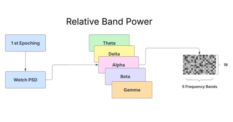
Fig. 2. Conceptual diagram of Relative Band Power (RBP) feature generation for a single epoch. Power Spectral Density (PSD) is computed using Welch's method. Power is then aggregated and normalized for five key frequency bands (Theta, Delta, Alpha, Beta, Gamma), producing a 19x5 feature map (19 channels x 5 frequency bands) used as input features

The relative band power was calculated by dividing the absolute power in each frequency band by the total power across all bands, resulting in a normalized measure that reduces the impact of inter-subject variability in overall signal amplitude.

1. Feature Reshaping: The extracted RBP features were reshaped into a 4D tensor (epochs, channels, frequency bands, 1) suitable for input to our convolutional neural network.
2. Data Splitting and Standardization: The dataset was split into training (80%) and testing (20%) sets, and standardization was applied to normalize the feature distributions, improving training stability and model performance.

The final input to our model had the shape (N, 19, 5, 1), representing N epochs, 19 EEG channels, five frequency bands, and one feature (relative band power).

Model Architecture

We propose a hybrid deep learning model combining Convolutional Neural Networks (CNNs) and Bidirectional Long Short-Term Memory (BiLSTM) networks for AD detection. The model processes Relative Band Power (RBP) features extracted from 2-second non-overlapping EEG epochs. These features are structured as input tensors of shape (19, 5, 1), representing 19 EEG channels, 5 canonical frequency bands (Delta: 0.5-4Hz, Theta: 4-8Hz, Alpha: 8-13Hz, Beta: 13-25Hz, Gamma: 25-45Hz) [Adjust band definitions if different], and a single feature dimension (power).

Fig. 3. Proposed CNN–BiLSTM classification architecture.

The architecture comprises:

1. CNN Feature Extractor:Processes the (19, 5, 1) input.
2. Block 1: Conv2D (32 filters, 3x3 kernel, L2 reg.) -> BatchNormalization -> ReLU -> MaxPooling2D (pool size (2, 1)), reducing the channel dimension while preserving frequency information.
3. Block 2: Conv2D (64 filters, 3x3 kernel, L2 reg.) -> BatchNormalization -> ReLU -> MaxPooling2D (pool size (2, 2)), downsampling both dimensions. This stage captures local spatial patterns across channels and spectral patterns within frequency bands.
4. Sequence Preparation: A Permute layer rearranges the CNN output dimensions to prioritize the frequency axis (batch, reduced_freqs, reduced_channels, filters), and A Reshape layer merges the channel and filter dimensions, creating a sequence input for the LSTM: (batch, sequence_length=reduced_freqs, features_per_step).
5. Sequential Modeling (BiLSTM): A Bidirectional LSTM layer (64 units, dropout, recurrent dropout, L2 reg.) processes the sequence of features derived from the frequency bands. This captures dependencies and contextual information across the spectral profile (e.g., relationships between alpha and beta band features). return_sequences=False is used for classification.
6. Classification Head: Dropout -> Dense (128 units, ReLU, L2 reg.) -> Dropout -> Dense (3 units, softmax activation) for final class prediction (A, F, C).

The model architecture is summarized in the following diagram:

Training Procedure

The model was trained using the Adam optimizer with a learning rate of 0.001 and a sparse categorical cross-entropy loss function. The dataset exhibited moderate class imbalance (Class A: ~42%, F: ~24%, C: ~34% of total epochs). Balanced class weights were computed using sklearn's 'balanced' mode and applied during training to mitigate this.

Training was regularized using L2 penalties on convolutional and dense layers, dropout in the LSTM and thick layers, and two callbacks: EarlyStopping (monitoring val_loss, patience 20, restoring best weights) and ReduceLROnPlateau (monitoring val_loss, factor 0.2, patience 7). Training ran for up to 100 epochs with a batch size of 128 on a dataset split into 80% training (~55k epochs) and 20% testing (~14k epochs). The final model weights were selected based on the lowest validation loss achieved during training.

Evaluation of the Proposed System

Experimental Setup

We evaluated our model using a rigorous experimental framework to assess its performance in classifying EEG signals from subjects with Alzheimer's, frontotemporal dementia, and healthy controls. The dataset was split into training (80%) and testing (20%) sets. We used accuracy, loss, and confusion matrices as our primary evaluation metrics.

The model is implemented using TensorFlow and Keras.

Results and Performance Analysis

The model achieved a test accuracy of 83.81% and a Log Loss of 0.4188. The Cohen's Kappa coefficient was 0.7520.

The per-class performance, as detailed in Table I, reveals generally robust results across all classes. Class C ('Control') achieved the highest precision (0.8751) and a high recall (0.8478), leading to the best F1-score (0.8612). Class A ('Alzheimer's') also performed well with balanced precision and recall (0.8407). Class F ('Frontotemporal Dementia') exhibited slightly lower metrics, with an accuracy of 0.7838 and recall of 0.8195 (F1-score: 0.8012).

Table I: Classification Report

This table summarizes the model's performance across three classes (A, F, C) in terms of precision, recall, and F1-score. The weighted and macro averages provide a holistic view of the model’s overall performance. Accuracy denotes the overall proportion of correctly classified instances.

Further analysis using the Area Under the Receiver Operating Characteristic Curve (AUC) with a One-vs-Rest strategy indicated excellent class separability at the probability level. The AUC scores were 0.9454 for Class A, 0.9558 for Class F, and 0.9625 for Class C, with a Macro Average AUC of 0.9546.

The normalized confusion matrix (Fig. Y - refer to the heatmap figure) provides insights into specific error patterns. The diagonal elements confirm the high recall values for each class (A: 0.84, F: 0.82, C: 0.85). The most notable misclassifications occurred where 13% of actual Class F instances were predicted as Class A, and 10% of actual Class C instances were predicted as Class A. Other misclassifications were less frequent (<= 8%). These results suggest that while the model effectively distinguishes the classes overall, there is some residual confusion, particularly in differentiating classes F and C from class A based on the learned spectral patterns.

Fig. 4. Normalized confusion matrix (recall) of the proposed CNN–BiLSTM model across classes A, F, and C..

Model Interpretability

The model's architecture suggests a tier-wise feature learning process. The CNN layers help to identify local patterns within the channel-frequency RBP representation (e.g., focal slowing, specific band power ratios). The BiLSTM subsequently models how these patterns relate across the frequency spectrum (delta through gamma). The observed high performance, particularly the high AUC scores, suggests the model successfully learned discriminative spectral profile characteristics for each class.

Observation

The hybrid CNN-BiLSTM model shows convergence during training: the loss decreases smoothly over epochs, and its accuracy improves until it plateaus, indicating effective learning of the EEG features. Training accuracy is slightly higher than the 83.81% test accuracy, implying good generalization. This suggests limited overfitting.

The CNN-BiLSTM architecture effectively combines spatial and temporal feature extraction. Convolutional layers learn spatial patterns from EEG band powers, while the BiLSTM captures temporal dynamics. The strong performance metrics (83.81% accuracy, Kappa 0.7520, macro AUC 0.9546) indicate excellent class discrimination.

Nonetheless, some class confusion remains. The overlaps in EEG spectral features for FTD and controls lead to misclassification. Cohen’s Kappa (0.7520) indicates substantial agreement, and the high AUC (0.9546) shows each class is well separated on average.

Conclusion

The main contribution of this work is a CNN-BiLSTM model that uses EEG spectral features to classify Alzheimer’s Disease, Frontotemporal Dementia, and healthy controls. The model’s high accuracy (83.81%), substantial Kappa (0.7520), and macro AUC (0.9546) demonstrate its effectiveness and potential utility for practical dementia screening. The results suggest that CNN-BiLSTM can successfully capture EEG patterns relevant to these conditions.

However, challenges remain, particularly class confusion between FTD and controls. This indicates that we need to incorporate more discriminative features. Future directions include adding advanced spectral ratios or connectivity biomarkers and training the model on more diverse and larger datasets.