How I Gained the Intuition Behind the ARIMA Model

Summary

In this article, we explore forecasting techniques with a focus on ARIMA, a powerful time series prediction model. Before diving into ARIMA, we first build a strong foundation by covering:

1. Types of Forecasting – Qualitative vs. Quantitative
2. Key Condition for Forecasting – Importance of stationarity and how to check it using the Augmented Dickey-Fuller (ADF) test
3. Quantitative Forecasting Methods – Naïve, Moving Average, and Exponential Smoothing
4. Breaking Down ARIMA – Understanding its components step by step:
   • AutoRegressive (AR) Model – How past values influence predictions, identified using Partial Autocorrelation Function (PACF)
   • Moving Average (MA) Model– How past errors affect predictions, identified using Autocorrelation Function (ACF)
   • ARMA Model – Combining AR and MA for better forecasting
   • ARIMA Model – Adding differencing to handle trends and achieve stationarity
5. Step-by-Step Implementation – A practical coding example using Python

By the end, you'll have a structured approach to understanding and implementing ARIMA for time series forecasting. Let’s dive in!

Why ARIMA?

I thought what concepts I am yet to explore in data. There were a lot!

But I noticed many data analytics job demand forecasting and thought why not. I understood the intuition behind it and wish there was a simpler way to put it all.

Moreover, learning forecasting seemed essential as it is used in variety of applications.

Where is ARIMA used?

• Stock Market: Predicts stock prices and market trends.
• Demand Forecasting: Helps businesses predict future product demand for inventory management.
• Sales Predictions: Forecasts revenue and sales trends to aid strategic planning.
• Economics: Used to predict inflation rates and other economic indicators.
• Weather Forecasting: Helps in predicting temperature, rainfall, and other climate patterns.
• Healthcare: Predicts disease outbreaks and healthcare resource demands.

I will quickly list out the topics I read before beginning ARIMA so you get the basics.

Part 1: Types of Forecasting techniques

• Qualitative
• Quantitative

We are going to focus in Quantitative techniques.

Part 2 : Common Condition to remember

Condition : Many forecasting models require the data to be stationary (statistical property like mean, variance should remain constant). If non-stationary data we do differencing (subtract current data from past).

So how can we know if a data is stationary or not?

We use Augumented Dickey Fuller Test

Part 3: Quantitative Forecasting Techniques

• Naive Method ( Today's value will be just like yesterday)
• Moving Average Method (Today's value will be average of last n days)
• Exponential smoothing (Today's value will be more influenced by the recent day than the days before)

Part 4: ARIMA.

A curse of learning by yourself is that you will realize how you should have already completed that it.

Similarly, when I jumped directly into learning the ARIMA model, I was bombarded with concepts like the order of p, d, q, lags, ARIMA (p, d, q), etc., all of which I had no clue about.

When I realized how I should have learnt this concept, I thought why not let others know what worked for me as it might work for others too. I came to understand that the components of ARIMA are individual mathematical forecasting models that should be understood separately first.

Here it goes...

Step 1: Understanding the AR (Auto Regressive) Model

What is the AR Model?

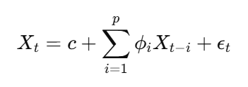
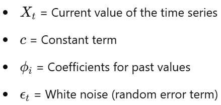
The Autoregressive (AR) model expresses a time series as a linear function of its past values. The number of past values used is denoted as p (the autoregressive order).

AR Model Equation:

where

So we have the equation, but what is p?

Yeah we know that it is the number of past values.

But how can we find the optimal number of past values that should be included in the formula?

For that we have, something called PACF (Partial Autocorrelation Function) that helps us determine the number of past values to be included in the AR model. Note: Only Basic intuition behind PACF and ACF is explained in this article

How PACF figures out p?

PACF removes indirect effects and shows only direct correlations between a time series and its past values.

In simple terms
Day 5 value can be directly influenced by Day 4 which is an example of direct effect
Day 5 value can be influenced by day 4 that itself is influenced by day 3 is an example of indirect effect.
So, by using PACF we can see the direct influences of day 1, day 2, day 3 and day 4 on day 5 value.

Still, how can we figure out p from PACF?

The p-value is the first significant lag where the PACF plot cuts off.

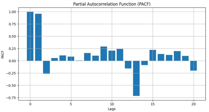
Image credits : GeeksforGeeks

Here p is the lag value that gave positive PACF value and dipped to zero right after it. So it is lag 2 therefore AR (2) component is the right solution.

Step 2: Understanding the MA (Moving Average) Model

This is just like AR model but there's a tiny difference, instead of past values, this model uses past errors.

What is the MA Model?

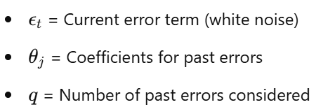
The Moving Average (MA) model expresses the time series as a linear function of past error terms. The number of past errors used is denoted as q (the moving average order).

MA Model Equation:

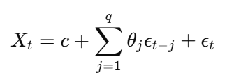
where:

So how do we find q?

• Just like before, here we use ACF (Autocorrelation Function) helps us to determine the number of past error terms to be included in the MA model.
• ACF measures correlations at different lags, including both direct and indirect effects.
• The q-value is the first significant lag where the ACF plot cuts off.

Step 3: Combining AR and MA Models - ARMA

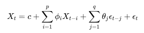
We now combine both of them to form a ARMA model. The ARMA (p, q) model is a combination of the AR and MA models, which accounts for both past values and past errors.

ARMA Model Equation:

Steps to Identify an ARMA Model:

1. Use PACF to determine (AR order).
2. Use ACF to determine (MA order).
3. Fit the ARMA model using these values.

Step 4: Introducing Differencing - ARIMA

Why Differencing is Needed?

Remember our common condition, that is why. If a time series has a trend (non-stationary behavior), AR and MA models alone won’t work effectively. To make the series stationary, we apply differencing.

So, what is differencing?

Differencing removes trends by subtracting each value from the previous one

Finally, hero of the story

ARIMA Model Equation:

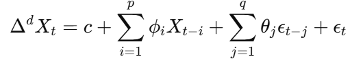
It is similar to the previous equation but only the delta d is included.
where

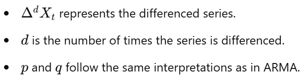
Steps to Identify an ARIMA Model:

1. Check for stationarity using the Augmented Dickey-Fuller (ADF) test.
2. If non-stationary, apply differencing until the series is stationary (find d).
3. Use PACF to determine p (AR order).
4. Use ACF to determine q (MA order).
5. Fit the ARIMA model using the identified values.

Example code by ChatGPT for reference

Step 1: Import Libraries

import numpy as np
import pandas as pd
import matplotlib.pyplot as plt
import statsmodels.api as sm
from statsmodels.tsa.stattools import adfuller
from statsmodels.graphics.tsaplots import plot_acf, plot_pacf
Step 2: Load and Visualize Data

# Sample monthly sales data (dummy example)
data = {
    "Month": pd.date_range(start="2018-01-01", periods=60, freq="M"),
    "Sales": [150, 160, 165, 170, 180, 190, 200, 210, 215, 220, 230, 240,
              250, 260, 270, 280, 290, 300, 310, 320, 325, 330, 340, 350,
              360, 370, 380, 390, 400, 410, 420, 430, 440, 450, 460, 470,
              480, 490, 500, 510, 520, 530, 540, 550, 560, 570, 580, 590,
              600, 610, 620, 630, 640, 650, 660, 670, 680, 690, 700, 710]
}

df = pd.DataFrame(data)
df.set_index("Month", inplace=True)

# Plot the time series
plt.figure(figsize=(10, 5))
plt.plot(df, marker="o", linestyle="-", label="Sales Data")
plt.xlabel("Year")
plt.ylabel("Sales")
plt.title("Monthly Sales Data")
plt.legend()
plt.show()
Observation: The data shows an increasing trend, so we may need differencing.

Step 3: Check for Stationarity
Before applying ARIMA, we check if the time series is stationary 
using the Augmented Dickey-Fuller (ADF) test.

# ADF Test
result = adfuller(df["Sales"])
print(f'ADF Statistic: {result[0]}')
print(f'p-value: {result[1]}')

# If p-value > 0.05, the data is non-stationary
If the p-value > 0.05, the series is not stationary, 
meaning we need to apply differencing.

Step 4: Apply Differencing (If Needed)

df_diff = df.diff().dropna()

# Plot differenced data
plt.figure(figsize=(10, 5))
plt.plot(df_diff, marker="o", linestyle="-", label="Differenced Sales Data")
plt.xlabel("Year")
plt.ylabel("Sales Difference")
plt.title("Differenced Monthly Sales Data")
plt.legend()
plt.show()

# ADF test on differenced data
result = adfuller(df_diff["Sales"])
print(f'ADF Statistic after Differencing: {result[0]}')
print(f'p-value: {result[1]}')
If the p-value < 0.05, the series is now stationary, 
and we can proceed with ARIMA.

Step 5: Identify ARIMA Parameters (p, d, q)
We use Autocorrelation Function (ACF) and Partial 
Autocorrelation Function (PACF) plots to 
determine the values of                         

Read More

Tags:

Previous Article

Benchmark CPUs Easily with the dkbench Docker image

Next Article

A coronavirus assembly inhibitor that targets the viral membrane protein

Related Posts

Becoming a Senior Developer - Tips from Clean Code

Feb 11, 2025  0

Why Europe needs to embrace its own tech alternatives

Feb 8, 2025  0

আপনি একজন প্রকৃত সফটওয়্যার ইঞ্জিনিয়ার হিসেবে সবসময় স...

Mar 7, 2025  0

Comments

Name

Email

Comment

Post Comment